Autoregressive models
We begin our study into generative modeling with autoregressive models. As before, we assume we are given access to a dataset of -dimensional datapoints . For simplicity, we assume the datapoints are binary, i.e., .
Representation
By the chain rule of probability, we can factorize the joint distribution over the -dimensions as
where denotes the vector of random variables with index less than .
The chain rule factorization can be expressed graphically as a Bayesian network.
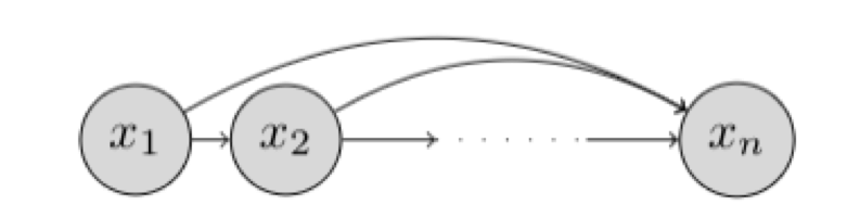
Such a Bayesian network that makes no conditional independence assumptions is said to obey the autoregressive property. The term autoregressive originates from the literature on time-series models where observations from the previous time-steps are used to predict the value at the current time step. Here, we fix an ordering of the variables and the distribution for the -th random variable depends on the values of all the preceeding random variables in the chosen ordering .
If we allow for every conditional to be specified in a tabular form, then such a representation is fully general and can represent any possible distribution over random variables. However, the space complexity for such a representation grows exponentially with .
To see why, let us consider the conditional for the last dimension, given by . In order to fully specify this conditional, we need to specify a probability for configurations of the variables . Since the probabilities should sum to 1, the total number of parameters for specifying this conditional is given by . Hence, a tabular representation for the conditionals is impractical for learning the joint distribution factorized via chain rule.
In an autoregressive generative model, the conditionals are specified as parameterized functions with a fixed number of parameters. That is, we assume the conditional distributions to correspond to a Bernoulli random variable and learn a function that maps the preceeding random variables to the mean of this distribution. Hence, we have
where denotes the set of parameters used to specify the mean function .
The number of parameters of an autoregressive generative model are given by . As we shall see in the examples below, the number of parameters are much fewer than the tabular setting considered previously. Unlike the tabular setting however, an autoregressive generative model cannot represent all possible distributions. Its expressiveness is limited by the fact that we are limiting the conditional distributions to correspond to a Bernoulli random variable with the mean specified via a restricted class of parameterized functions.
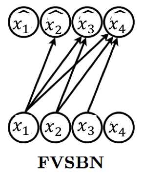
In the simplest case, we can specify the function as a linear combination of the input elements followed by a sigmoid non-linearity (to restrict the output to lie between 0 and 1). This gives us the formulation of a fully-visible sigmoid belief network (FVSBN).
where denotes the sigmoid function and denote the parameters of the mean function. The conditional for variable requires parameters, and hence the total number of parameters in the model is given by . Note that the number of parameters are much fewer than the exponential complexity of the tabular case.
A natural way to increase the expressiveness of an autoregressive generative model is to use more flexible parameterizations for the mean function e.g., multi-layer perceptrons (MLP). For example, consider the case of a neural network with 1 hidden layer. The mean function for variable can be expressed as
where denotes the hidden layer activations for the MLP and are the set of parameters for the mean function . The total number of parameters in this model is dominated by the matrices and given by .
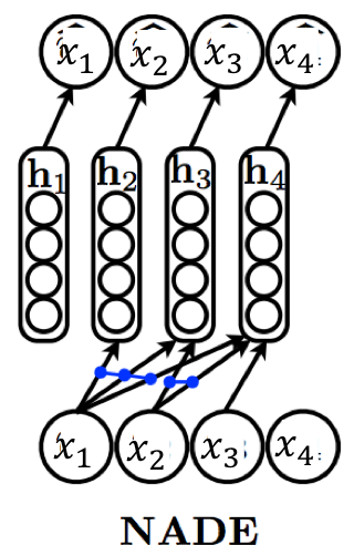
The Neural Autoregressive Density Estimator (NADE) provides an alternate MLP-based parameterization that is more statistically and computationally efficient than the vanilla approach. In NADE, parameters are shared across the functions used for evaluating the conditionals. In particular, the hidden layer activations are specified as
where is the full set of parameters for the mean functions . The weight matrix and the bias vector are shared across the conditionals. Sharing parameters offers two benefits:
-
The total number of parameters gets reduced from to [readers are encouraged to check!].
-
The hidden unit activations can be evaluated in time via the following recursive strategy:
with the base case given by .
Extensions to NADE
The RNADE algorithm extends NADE to learn generative models over real-valued data. Here, the conditionals are modeled via a continuous distribution such as a equi-weighted mixture of Gaussians. Instead of learning a mean function, we know learn the means and variances of the Gaussians for every conditional. For statistical and computational efficiency, a single function outputs all the means and variances of the Gaussians for the -th conditional distribution.
Notice that NADE requires specifying a single, fixed ordering of the variables. The choice of ordering can lead to different models. The EoNADE algorithm allows training an ensemble of NADE models with different orderings.
Learning and inference
Recall that learning a generative model involves optimizing the closeness between the data and model distributions. One commonly used notion of closeness in the KL divergence between the data and the model distributions.
Before moving any further, we make two comments about the KL divergence. First, we note that the KL divergence between any two distributions is asymmetric. As we navigate through this chapter, the reader is encouraged to think what could go wrong if we decided to optimize the reverse KL divergence instead. Secondly, the KL divergences heavily penalizes any model distribution which assigns low probability to a datapoint that is likely to be sampled under . In the extreme case, if the density evaluates to zero for a datapoint sampled from , the objective evaluates to .
Since does not depend on , we can equivalently recover the optimal parameters via maximizing likelihood estimation.
Here, is referred to as the log-likelihood of the datapoint with respect to the model distribution .
To approximate the expectation over the unknown , we make an assumption: points in the dataset are sampled i.i.d. from . This allows us to obtain an unbiased Monte Carlo estimate of the objective as
The maximum likelihood estimation (MLE) objective has an intuitive interpretation: pick the model parameters that maximize the log-probability of the observed datapoints in .
In practice, we optimize the MLE objective using mini-batch gradient ascent. The algorithm operates in iterations. At every iteration , we sample a mini-batch of datapoints sampled randomly from the dataset () and compute gradients of the objective evaluated for the mini-batch. These parameters at iteration are then given via the following update rule
where and are the parameters at iterations and respectively, and is the learning rate at iteration . Typically, we only specify the initial learning rate and update the rate based on a schedule. Variants of stochastic gradient ascent, such as RMS prop and Adam, employ modified update rules that work slightly better in practice.
From a practical standpoint, we must think about how to choose hyperaparameters (such as the initial learning rate) and a stopping criteria for the gradient descent. For both these questions, we follow the standard practice in machine learning of monitoring the objective on a validation dataset. Consequently, we choose the hyperparameters with the best performance on the validation dataset and stop updating the parameters when the validation log-likelihoods cease to improve1.
Now that we have a well-defined objective and optimization procedure, the only remaining task is to evaluate the objective in the context of an autoregressive generative model. To this end, we substitute the factorized joint distribution of an autoregressive model in the MLE objective to get
where now denotes the collective set of parameters for the conditionals.
Inference in an autoregressive model is straightforward. For density estimation of an arbitrary point , we simply evaluate the log-conditionals for each and add these up to obtain the log-likelihood assigned by the model to . Since we know conditioning vector , each of the conditionals can be evaluated in parallel. Hence, density estimation is efficient on modern hardware.
Sampling from an autoregressive model is a sequential procedure. Here, we first sample , then we sample conditioned on the sampled , followed by conditioned on both and and so on until we sample conditioned on the previously sampled . For applications requiring real-time generation of high-dimensional data such as audio synthesis, the sequential sampling can be an expensive process. Later in this course, we will discuss how parallel Wavenet, an autoregressive model sidesteps this expensive sampling process.
Finally, an autoregressive model does not directly learn unsupervised representations of the data. In the next few set of lectures, we will look at latent variable models (e.g., variational autoencoders) which explicitly learn latent representations of the data.
Footnotes
-
Given the non-convex nature of such problems, the optimization procedure can get stuck in local optima. Hence, early stopping will generally not be optimal but is a very practical strategy. ↩